

Blog
Sensor Virtualization using Artificial Intelligence & Machine Learning
Navigation
NavigationIntroduction
Virtualization is revolutionizing the automotive industry, enabling the development and validation of software-defined vehicles (SDV) [1]. Virtualization allows the creation of a simulated environment, wherein various components of a vehicle can be developed and tested much early. Sensor virtualization is a technique that uses data from one set of real sensors and/or other parameters to estimate the outcome of another set of sensors [2]. Virtual sensors are implemented in complete software domain as against the physical real sensors.
Sensor virtualization is used in the following scenarios:
- In safety-critical applications, virtual sensors can be used to provide accurate data when a real sensor is giving erratic readings or is unavailable. By leveraging patterns in data from existing sensors through machine learning, it’s possible to infer data of an unavailable physical sensor. One could also use virtual sensors to augment the readings from real sensors.
- SDV era will see more software and less hardware. There is a tendency to move more hardware implementations to software. Thus, using a virtual sensor instead of real sensor have many benefits, such as less wiring, less weight, flexibility in sensor deployment, and enabling applications in environments where some sensors can’t be used directly. Also, there is a trend of sensor consolidation to reduce the number of sensors in the vehicle.
Virtual sensors have applications in industrial monitoring and maintenance, healthcare, precision agriculture, smart cities, and automobiles. In this blog report, we will discuss about sensor virtualization and its benefits with an example.
Sensor virtualization using machine learning
Artificial intelligence and machine learning (AI ML) models can identify the relationships and correlations between observed variable readings from real sensors and other parameters. Feature selection techniques are first applied to determine the parameters that serve as strong predictors for the target virtual sensor reading [3]. Machine learning models are then trained on selected historical data from the available sensors and other parameters to capture temporal and spatial patterns effectively. Regression models, such as linear regression, random forests, gradient boosting machine, and multi-layer perceptron neural network, are particularly well-suited for predicting the sensor reading based on input data from related physical sensors and other parameters. When the sensor output depends on time-series data, sequence models such as long short-term memory are more suitable.
Digital twin technology, which involves creating a virtual replica of a physical system, is being widely adopted in many domains. By leveraging digital twins, manufacturers can simulate, analyse and optimize physical system’s performance, maintenance, and service life. In the automotive industry, this technology not only enhances the design of electronic control units (ECUs) and sensors in the vehicles but also aids in the development of predictive maintenance strategies, thereby reducing operational costs and improving reliability. For applications such as fault detection, machine learning models are trained on physical sensor data to establish a baseline. When data from physical sensors diverge from the baseline, it can signal an anomaly. This is common in applications like turbo-machinery monitoring, where a virtual sensor baseline helps identify when physical sensors or machinery may be malfunctioning [4].
A workflow for sensor virtualization using machine learning
The sensor virtualization process involves different stages: Feature selection and model training with selected input features, Prediction using the trained model, Performance evaluation and model selection, and Embedded implementation as shown in Figure 1. Each of these stages is explained below.
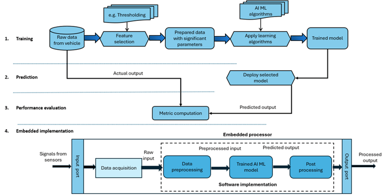
Figure 1: Sensor virtualization workflow
- Feature selection and model training - The dataset is first pre-processed to remove data samples with missing values and the data is normalized. To reduce computational complexity, various feature selection techniques are applied. The AI ML models are then trained with the significant parameters to predict the target sensor output. The dataset is split into two, training and test datasets. Each potential AI ML model is trained on the training dataset with and without feature selection. A part of the training dataset is used for validation of the model during training. The model parameters are adjusted to get the best validation results.
- Prediction using test dataset - Once the trained model is available, it is fed with the data samples from the test dataset. The predicted outputs for the unseen input data are collected. For each trained AI ML model, the prediction process is carried out for the same test dataset to compare the performance of different AI ML models.
- Performance evaluation and model selection - The performance of models is evaluated by comparing the predicted outputs with the actual target sensor outputs. A comprehensive set of error metrics are computed for performance evaluation. Apart from the metrics used to assess the accuracy of prediction, the training and inference times of each model is also computed to assess the model's efficiency and robustness. The model demonstrating high prediction accuracy, with minimal input features, and lower inference time can be chosen as the optimal one.
- Embedded implementation - The chosen trained model is then implemented on an embedded platform like an ECU. The embedded processor receives the raw inputs (selected sensors’ values and certain parameters over ECU interfaces) at regular intervals. They are pre-processed and fed to the trained model which predicts the target sensor value. The sampling rate of inputs are decided based on the inference time of the model in embedded platform.
Case study: Virtualization of motor temperature sensor
Dataset
The dataset used in this study is sourced from Kaggle [5] and consists of 185 hours of recordings from a permanent magnet synchronous motor (PMSM), sampled at a frequency of 2 Hz (one measurement every 0.5 seconds), resulting in approximately 1.33 million samples. The data is organized into 69 sessions, each identified by a unique ‘profile id’ indicating different operational scenarios. The dataset includes 12 variables, 11 input features and one target variable, the permanent magnet temperature (in °C), which is crucial for monitoring motor performance and preventing overheating. The input features capture various aspects of the motor’s operation, including motor speed, torque, currents and voltages in the d/q coordinates, coolant temperature, stator winding, and stator tooth temperatures. Each row in the dataset represents a specific operational state, capturing fluctuations in motor speed, thermal variations, and dynamic characteristics. The samples collected under diverse operational scenarios make the dataset valuable for developing predictive models.
Predictive modelling of motor temperature
Four different AI ML models were implemented in Python using scikit-learn machine learning library. They were trained on the dataset after applying various feature selection techniques. 75% of the dataset was used for training and the rest was used for performance evaluation. The parameters of the models as listed in Table 1 were tuned to get the best performance. The prediction accuracies of the models for different feature extraction methods are displayed in the bar chart shown in Figure 2. The prediction accuracy is given by 100-MAPE, where MAPE is mean absolute percentage error. It is noted that the random forest regressor outperforms other models with a prediction accuracy over 99%. The numbers marked above the bars give the number of features selected. With only three input features selected through thresholding technique, the random forest regression predicts the motor temperature with high accuracy. The three features are motor speed, stator yoke temperature, and d-component of voltage. The importance score of each input feature in predicting the motor temperature is derived through feature importance method and is shown in Figure 3. It is observed that the motor speed and stator yoke temperature highly influence the motor temperature.
| Model | Parameters |
| Random Forest Regressor | n_estimators=10 (number of trees) |
| Gradient Boosting Regressor | n_estimators=100 (number of boosting stages) |
| Multilayer Perceptron (MLP Regressor) | hidden_layer_sizes=(100, 50) (two hidden layers: 100 and 50 neurons) |
| max_iter =1000 (maximum iterations) |
Table 1: Model parameters
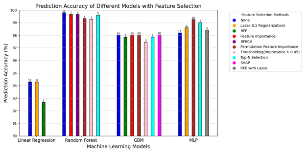
Figure 2: Prediction accuracies of AI ML models using various feature selection methods Table
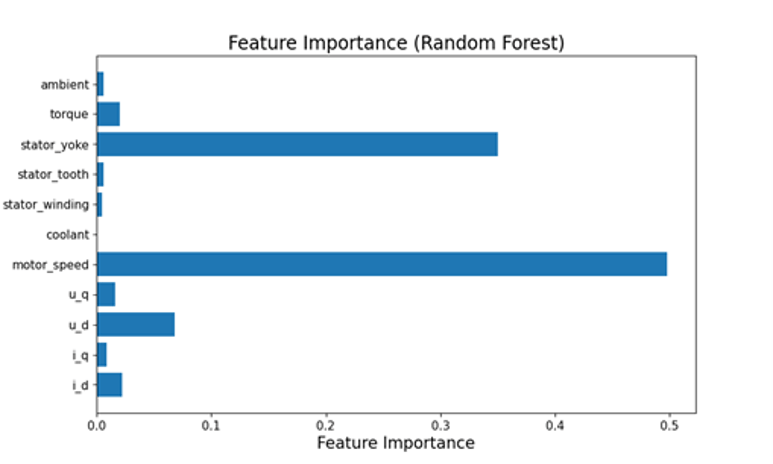
Figure 3: Importance scores of different input features for random forest model
The scatter plot showing actual and predicted temperature values using test data set for the random forest model is shown in Figure 4. It is observed that most of the points lie near the ideal line which demonstrates the efficacy of the model. Table 2 displays the error metrics computed for the random forest regression model with and without feature selection methods applied. The error metrics, remain consistently low across methods with different number of features selected, demonstrating high predictive accuracy. Although there is a slight drop in performance when fewer features are selected, the reduced number of features however results in faster computations. The three-quality metrics achieve nearly their maximum value of 1, indicating a perfect model fit.
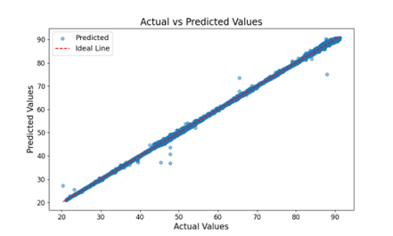
Figure 4: Scatter plot of actual versus predicted temperature values in testing phase for random forest model
|
Metrics |
None (11) |
Feature |
Recursive Feature Elimination with Cross Validation |
Top N |
Permutation |
Thresholding |
|
Mean Squared Error (MSE) |
0.06 |
0.1 |
0.1 |
0.11 |
0.26 |
0.33 |
|
Mean Squared Logarithmic Error (MSLE) |
0 |
0 |
0 |
0 |
0 |
0 |
|
Mean Absolute Error (MAE) |
0.1 |
0.16 |
0.16 |
0.18 |
0.28 |
0.32 |
|
Mean Absolute Percentage Error (MAPE) |
0.19% |
0.32% |
0.33% |
0.38% |
0.65% |
0.72% |
|
Median Absolute Error (MedAE) |
0.04 |
0.07 |
0.07 |
0.09 |
0.12 |
0.13 |
|
Symmetric Mean Absolute Percentage Error (SMAPE) |
0.19% |
0.32% |
0.33% |
0.38% |
0.65% |
0.72% |
|
R-squared (R²) |
1 |
0.99 |
0.99 |
0.99 |
0.99 |
0.99 |
|
Adjusted R-Squared |
1 |
0.99 |
0.99 |
0.99 |
0.99 |
0.99 |
|
Explained Variance Score |
1 |
0.99 |
0.99 |
0.99 |
0.99 |
0.99 |
|
Max Error |
12.87 |
13.79 |
12.72 |
12.25 |
12.37 |
11.13 |
|
Prediction accuracy (100-MAPE) |
99.81% |
99.67% |
99.66% |
99.61% |
99.34% |
99.27% |
Table 2: Performance metrics computed for random forest regression model with different feature selection techniques. The numbers within parenthesis indicate the number of features selected.
Realization on Raspberry Pi
The random forest prediction model, utilizing three significant input features (motor speed, stator yoke and u_d) was deployed on a Raspberry Pi 4 model B [6] embedded development board. The board was connected to a PC via Ethernet for two-way data communication using the SOME/IP protocol [7]. The experimental setup is shown in Figure 5. In this setup, the data values of the three input features were transmitted from the PC to the board and the predicted temperature value was received. A screenshot of data communication with embedded virtual sensor, as displayed on the PC monitor, is shown in the figure. The arrows point to the transmission and reception times. The total time for data transfer and prediction is approximately 50 ms, with the regression model taking only 5 ms to predict the temperature based on the input data.
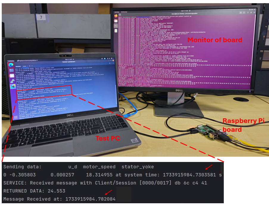
Figure 5: Virtual sensor experimental setup and screenshot of data communication
Outcomes and benefits
The outcomes of this case study demonstrate the effectiveness of machine learning techniques for accurately predicting the target sensor output. By evaluating multiple models, including Linear Regression, Random Forest, Gradient Boosting, and Multi-Layer Perceptron, the Random Forest model emerged as the most effective, achieving over 99% prediction accuracy with just three carefully selected features. When input features are large in number, feature selection plays a critical role in enhancing model performance, computational efficiency, and reliability by removing the irrelevant features. The study further reveals the suitability of embedded implementation of the AI ML model for real-time sensing applications due to its low inference time. The embedded virtual sensor on a Raspberry Pi can process approximately 20 inputs per second.
Conclusion
A comprehensive framework was outlined for deploying predictive models to design digital twins, enhancing reliability, efficiency, and operational longevity. The case study demonstrated how to construct a virtual sensor from historical data using machine learning, showcasing its ability to provide outputs close to real world. The realization of virtual sensors on embedded platforms further highlighted their feasibility for real-time deployment. Tata Elxsi is supporting OEMs and Tier Ones in virtualizing sensors for cost-effectiveness and enhanced reliability.
References
- John Makin and Gregor Matenaer, “Virtualization: Revolutionizing the software-defined vehicle landscape”, May 19, 2023 (Blog: Achieving the benefits of SDVs using virtualization | Luxoft)
- Dominik Martin, Niklas Kuhl and Gerhard Satzger, “Virtual sensors”, Business & Information Systems Engineering, vol. 63, pp. 315-323, March 2021.
- Liu H., “Feature selection”, Encyclopedia of Machine Learning, Springer, pp. 402-406, 2011.
- Sachin Shetty, Valentina Gori, Gianni Bagni and Giacomo Veneri, “Sensor Virtualization for anomaly detection of turbo-machinery sensors – An industrial application”, Engineering Proceedings, MDPI, vol. 39, no. 1, 2023.
- Electric motor temperature dataset: https://www.kaggle.com/datasets/wkirgsn/electric-motor-temperature
- Raspberry Pi 4 Model B specification: https://www.raspberrypi.com/products/raspberry-pi-4-model-b/specifications/
- AUTOSAR SOME/IP protocol specification: https://www.autosar.org/fileadmin/standards/R22-11/FO/AUTOSAR_PRS_SOMEIPProtocol.pdf


